SQL Performance Analyzer in Oracle Database 11g Release 1
The concept of SQL tuning sets, along with the
DBMS_SQLTUNE package to manipulate them, was introduced in Oracle 10g as part of the
Automatic SQL Tuning
functionality. Oracle 11g makes further use of SQL tuning sets with the
SQL Performance Analyzer, which compares the performance of the
statements in a tuning set before and after a database change. The
database change can be as major or minor as you like, such as:
- Database, operating system, or hardware upgrades.
- Database, operating system, or hardware configuration changes.
- Database initialization parameter changes.
- Schema changes, such as adding indexes or materialized views.
- Refreshing optimizer statistics.
- Creating or changing SQL profiles.
Unlike
Database Replay,
the SQL Performance Analyzer does not try and replicate the workload on
the system. It just plugs through each statement gathering performance
statistics.
The SQL Performance Analyzer can be run manually using the
DBMS_SQLPA package or using Enterprise Manager. This article gives an overview of both methods.
Setting Up the Test
The SQL performance analyzer requires SQL tuning sets, and SQL tuning
sets are pointless unless they contain SQL, so the first task should be
to issue some SQL statements. We are only trying to demonstrate the
technology, so the example can be really simple. The following code
creates a test user called
SPA_TEST_USER.
CONN / AS SYSDBA

CREATE USER spa_test_user IDENTIFIED BY spa_test_user
  QUOTA UNLIMITED ON users;

GRANT CONNECT, CREATE TABLE TO spa_test_user;
Next, connect to the test user and create a test table called
MY_OBJECTS using a query from the
ALL_OBJECTS view.
CONN spa_test_user/spa_test_user

CREATE TABLE my_objects AS
  SELECT * FROM all_objects;

EXEC DBMS_STATS.gather_table_stats(USER, 'MY_OBJECTS', cascade => TRUE);
This schema represents our "before" state. Still logged in as the test user, issue the following statements.
SELECT COUNT(*) FROM my_objects WHERE object_id <= 100;
SELECT object_name FROM my_objects WHERE object_id = 100;
SELECT COUNT(*) FROM my_objects WHERE object_id <= 1000;
SELECT object_name FROM my_objects WHERE object_id = 1000;
SELECT COUNT(*) FROM my_objects WHERE object_id BETWEEN 100 AND 1000;
Notice, all statements make reference to the currently unindexed
OBJECT_ID column. Later we will be indexing this column to create our changed "after" state.
The select statements are now in the shared pool, so we can start creating an SQL tuning set.
Creating SQL Tuning Sets using the DBMS_SQLTUNE Package
The
DBMS_SQLTUNE package contains procedures and
functions that allow us to create, manipulate and drop SQL tuning sets.
The first step is to create an SQL tuning set called
spa_test_sqlset using the
CREATE_SQLSET procedure.
CONN / AS SYSDBA

EXEC DBMS_SQLTUNE.create_sqlset(sqlset_name => 'spa_test_sqlset');
Next, the
SELECT_CURSOR_CACHE table function is used to retrieve a cursor containing all SQL statements that were parsed by the
SPA_TEST_USER schema and contain the word "my_objects". The resulting cursor is loaded into the tuning set using the
LOAD_SQLSET procedure.
DECLARE
  l_cursor  DBMS_SQLTUNE.sqlset_cursor;
BEGIN
  OPEN l_cursor FOR
     SELECT VALUE(a)
     FROM   TABLE(
              DBMS_SQLTUNE.select_cursor_cache(
                basic_filter   => 'sql_text LIKE ''%my_objects%'' and parsing_schema_name = ''SPA_TEST_USER''',
                attribute_list => 'ALL')
            ) a;


  DBMS_SQLTUNE.load_sqlset(sqlset_name     => 'spa_test_sqlset',
                           populate_cursor => l_cursor);
END;
/
The
DBA_SQLSET_STATEMENTS view allows us to see which statements have been associated with the tuning set.
SELECT sql_text
FROM   dba_sqlset_statements
WHERE  sqlset_name = 'spa_test_sqlset';

SQL_TEXT
--------------------------------------------------------------------------------
SELECT object_name FROM my_objects WHERE object_id = 100
SELECT COUNT(*) FROM my_objects WHERE object_id <= 100
SELECT COUNT(*) FROM my_objects WHERE object_id BETWEEN 100 AND 1000
SELECT COUNT(*) FROM my_objects WHERE object_id <= 1000
SELECT object_name FROM my_objects WHERE object_id = 1000

5 rows selected.

SQL>
Now we have an SQL tuning set, we can start using the SQL performance analyzer.
Running the SQL Performance Analyzer using the DBMS_SQLPA Package
The
DBMS_SQLPA package is the PL/SQL API used to manage the SQL performance ananlyzer. The first step is to create an analysis task using the
CREATE_ANALYSIS_TASK function, passing in the SQL tuning set name and making a note of the resulting task name.
CONN / AS SYSDBA

VARIABLE v_task VARCHAR2(64);
EXEC :v_task :=  DBMS_SQLPA.create_analysis_task(sqlset_name => 'spa_test_sqlset');

PL/SQL procedure successfully completed.

SQL> PRINT :v_task

V_TASK
--------------------------------------------------------------------------------
TASK_122

SQL>
Next, use the
EXECUTE_ANALYSIS_TASK procedure to execute
the contents of the SQL tuning set against the current state of the
database to gather information about the performance before any
modifications are made. This analysis run is named
before_change.
BEGIN
  DBMS_SQLPA.execute_analysis_task(
    task_name       => :v_task,
    execution_type  => 'test execute',
    execution_name  => 'before_change');
END;
/
Now we have the "before" performance information, we need to make a
change so we can test the "after" performance. For this example we will
simply add an index to the test table on the
OBJECT_ID column. In a new SQL*Plus session create the index using the following statements.
CONN spa_test_user/spa_test_user

CREATE INDEX my_objects_index_01 ON my_objects(object_id);

EXEC DBMS_STATS.gather_table_stats(USER, 'MY_OBJECTS', cascade => TRUE);
Now, we can return to our original session and test the performance after the database change. Once again use the
EXECUTE_ANALYSIS_TASK procedure, naming the analysis task "after_change".
BEGIN
  DBMS_SQLPA.execute_analysis_task(
    task_name       => :v_task,
    execution_type  => 'test execute',
    execution_name  => 'after_change');
END;
/
Once the before and after analysis tasks are complete, we must run a
comparison analysis task. The following code explicitly names the
analysis tasks to compare using name-value pairs in the
EXECUTION_PARAMS parameter. If this is ommited, the latest two analysis runs are compared.
BEGIN
  DBMS_SQLPA.execute_analysis_task(
    task_name        => :v_task,
    execution_type   => 'compare performance',
    execution_params => dbms_advisor.arglist(
                          'execution_name1',
                          'before_change',
                          'execution_name2',
                          'after_change')
    );
END;
/
With this final analysis run complete, we can check out the comparison report using the
REPORT_ANALYSIS_TASK function. The function returns a CLOB containing the report in 'TEXT', 'XML' or 'HTML' format. Its usage is shown below.
Note. Oracle 11gR2 also includes an 'ACTIVE' format that looks more like the Enterprise Manager output.
SET PAGESIZE 0
SET LINESIZE 1000
SET LONG 1000000
SET LONGCHUNKSIZE 1000000
SET TRIMSPOOL ON
SET TRIM ON

SPOOL /tmp/execute_comparison_report.htm

SELECT DBMS_SQLPA.report_analysis_task(:v_task, 'HTML', 'ALL')
FROM   dual;

SPOOL OFF
An example of this file for each available type is shown below.
- TEXT
- HTML
- XML
- ACTIVE
- Active HTML available in 11gR2 requires a download of Javascript
libraries from an Oracle website, so must be used on a PC connected to
the internet.
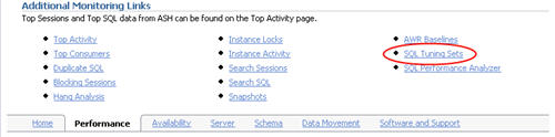
Creating SQL Tuning Sets using Enterprise Manager
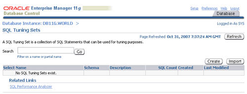
Click on the "SQL Tuning Sets" link towards the bottom of the "Performance" tab.
On the "SQL Tuning Sets" screen, click the "Create" button.
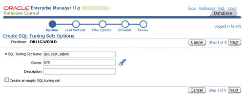
Enter a name for the SQL tuning set and click the "Next" button.
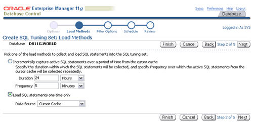
Select the "Load SQL statements one time only" option, select the
"Cursor Cache" as the data source, then click the "Next" button.
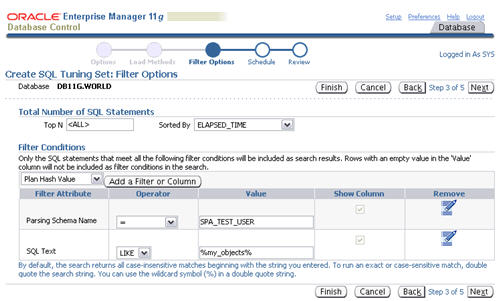
Set the appropriate values for the "Parsing Schema Name" and "SQL
Text" filter attributes, remove any extra attributes by clicking their
remove icons, then click the "Next" button.
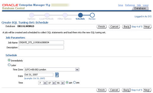
Accept the immediate schedule by clicking the "Next" button.
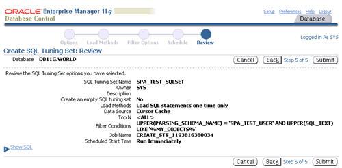
Assuming the review information looks correct, click the "Submit" button.
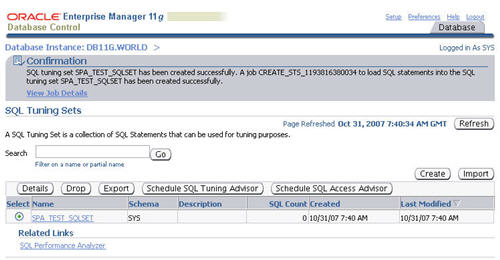
The "SQL Tuning Sets" screen shows the confirmation of the tuning set creation and the scheduled job to populate it.
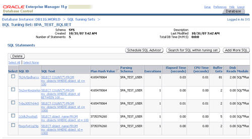
Once the population job completes, clicking on the SQL tuning set displays its contents.
Now we have an SQL tuning set, we can start using the SQL performance analyzer.
Running the SQL Performance Analyzer using Enterprise Manager
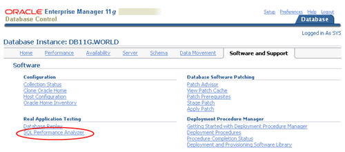
Click the "SQL Performance Analayzer" link on the "Software and Support" tab.
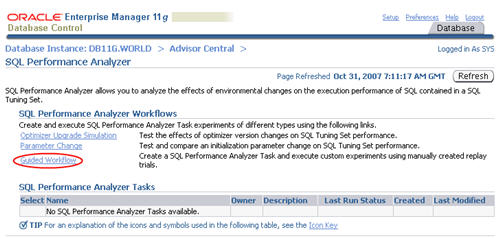
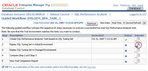
Click the "Guided Workflow" link on the "SQL Performance Analayzer" screen.
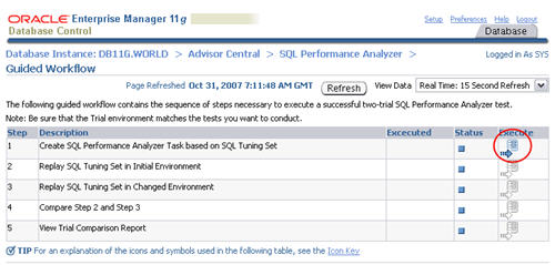
Click the execute icon on the first step to create the SQL Performance Analyzer task.
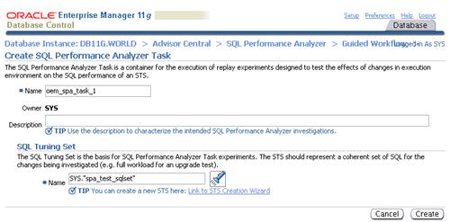
Enter a name for the SPA task, select the SQL tuning set to associate with it, then click the "Create" button.
When the status of the previous step becomes a green tick, click the
execute icon on the second step to capture the SQL tuning set
performance information of the "before" state.
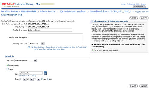
Enter a "Replay Trial Name" of "before_change", check the "Trial
environment established" checkbox, then click the "Submit" button.
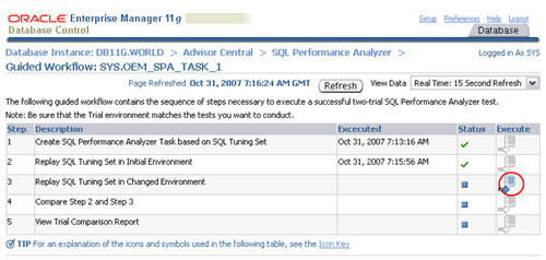
When the status of the previous step becomes a green tick, click the
execute icon on the third step to capture the SQL tuning set performance
information of the "after" state.
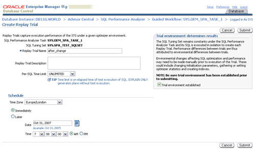
Alter the state of the database by creating an index on the
OBJECT_ID column of the test table.
CONN spa_test_user/spa_test_user@prod

CREATE INDEX my_objects_index_01 ON my_objects(object_id);

EXEC DBMS_STATS.gather_table_stats(USER, 'MY_OBJECTS', cascade => TRUE);
Enter a "Replay Trial Name" of "after_change", check the "Trial
environment established" checkbox, then click the "Submit" button.
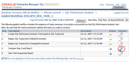
When the status of the previous step becomes a green tick, click the
execute icon on the forth step to run a comparison analysis task.
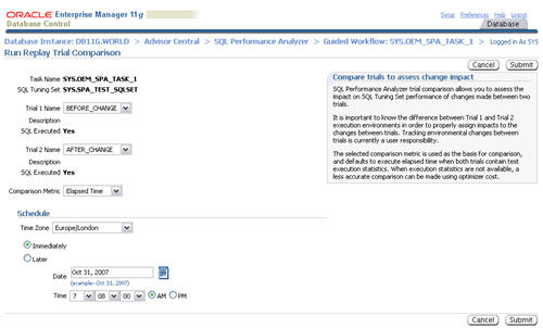
Accept the default "Trial 1 Name" and "Trial 2 Name" settings by clicking the "Submit" button.
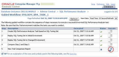
When the status of the previous step becomes a green tick, click the
execute icon on the fifth step to view the comparison report.
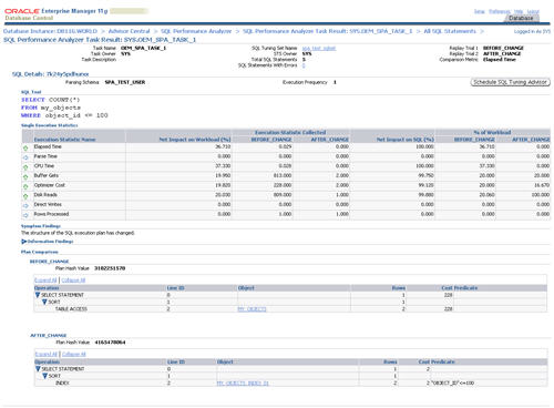
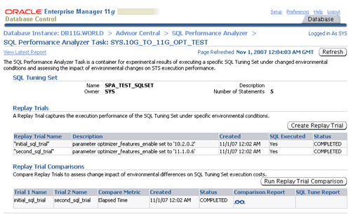
The resulting page contains the comparison report for the SQL Performance Analyzer task.
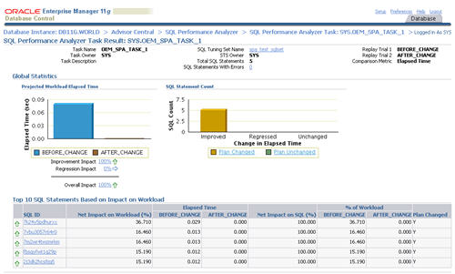
Clicking on a specific SQL ID displays the statement specific results, along with the before and after execution plans.
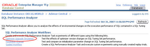
Optimizer Upgrade Simulation
The SQL Performance Analyzer allows you to test the affects of
optimizer version changes on SQL tuning sets. Click the "Optimizer
Upgrade Simulation" link on the "SQL Performance Analyzer" page.
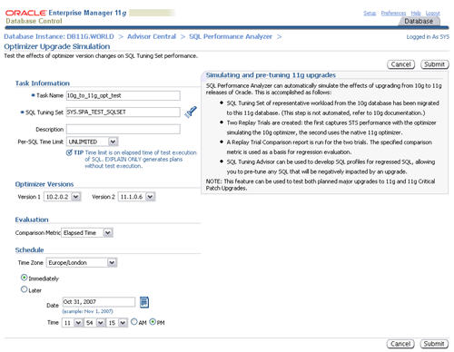
Enter a task name, select the two optimizer versions to compare, then click the "Submit" button.
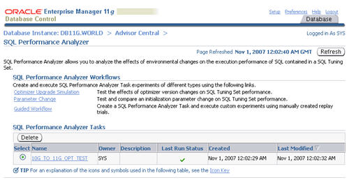
The task is listed in the "SQL Performance Analyzer Tasks" section.
Refresh the page intermittently until the task status becomes a green
tick, then click on the task name.
The resulting screen shows details of the selected task. Click on the
"Comparison Report" classes icon allows you to view the comparison
report.
Parameter Change
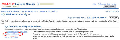
The SQL Performance Analyzer provides a shortcut for setting up tests
of initialization parameter changes on SQL tuning sets. Click the
"Parameter" link on the "SQL Performance Analyzer" page.
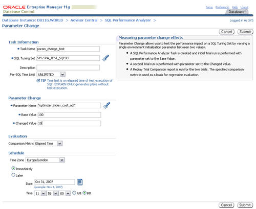
Enter a task name and the parameter you wish to test. Enter the base and changed value, then click the "Submit" button.
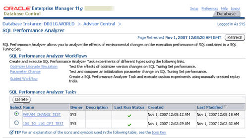
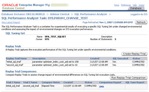
The task is listed in the "SQL Performance Analyzer Tasks" section.
Refresh the page intermittently until the task status becomes a green
tick, then click on the task name.
The resulting screen shows details of the selected task. Click on the
"Comparison Report" classes icon allows you to view the comparison
report.
Transferring SQL Tuning Sets
In the examples listed above, the tests have been performed on the
same system. In reality you are more likely to want to create a tuning
set on your production system, then run the SQL Performance Analyzer
against it on a test system. Fortunately, the
DBMS_SQLTUNE package allows you to transport SQL tuning sets by storing them in a staging table.
First, create the staging table using the
CREATE_STGTAB_SQLSET procedure.
CONN sys/password@prod AS SYSDBA

BEGIN
  DBMS_SQLTUNE.create_stgtab_sqlset(table_name      => 'SQLSET_TAB',
                                    schema_name     => 'SPA_TEST_USER',
                                    tablespace_name => 'USERS');
END;
/
Next, use the
PACK_STGTAB_SQLSET procedure to export SQL tuning set into the staging table.
BEGIN
  DBMS_SQLTUNE.pack_stgtab_sqlset(sqlset_name          => 'SPA_TEST_SQLSET',
                                  sqlset_owner         => 'SYS',
                                  staging_table_name   => 'SQLSET_TAB',
                                  staging_schema_owner => 'SPA_TEST_USER');
END;
/
Once the SQL tuning set is packed into the staging table, the table
can be transferred to the test system using Datapump, Export/Import or
via a database link. Once on the test system, the SQL tuning set can be
imported using the
UNPACK_STGTAB_SQLSET procedure.
BEGIN
  DBMS_SQLTUNE.unpack_stgtab_sqlset(sqlset_name          => '%',
                                    sqlset_owner         => 'SYS',
                                    replace              => TRUE,
                                    staging_table_name   => 'SQLSET_TAB',
                                    staging_schema_owner => 'SPA_TEST_USER');
END;
/
The SQL tuning set can now be used with the SQL Performance Analyzer on the test system.
For more information see: